Generative Adversarial Networks

In this blog post, we are going to discuss about a relatively new area of machine learning known as Generative Adversarial Networks or GAN. GANs were introduced to the world by a seminal work by Dr. Ian Goodfellow. In this post, we will look at the background of GANs, intuition, a little peek into the mathematics. Followed by this, we will illustrate GANs using a small toy example.

Post URL – https://interestedintech.wordpress.com/2017/04/03/generative-adversarial-networks

Introduction

Generative Adversarial Networks (GANs) fall under the branch of unsupervised machine learning. Mentioning that, there are no labels required for this technique. The concept of GANs can be summarized from its name itself. Let’s look at each word.

1. Generative – GANs fall under a class of machine learning known as generative models. Few other examples of generative models are gaussian mixture models, hidden markov models, naive bayes etc. For more information, please visit this link. We will see generative models below.
2. Adversarial –  Adversary according to English dictionary means “opponent in a conflict or dispute”. In the context of GANs adversarial refers to using two competing models to generate good data. These models are called as generator & discriminator which we will go into details in a little bit.
3. Network – As the name suggests, the models generally are neural networks.

Let us first see the two kinds of machine learning models.

Discriminative Models –  Discriminative models are used to model the dependence of unobserved variable y on the observered variable x. This is used to model the conditional probabilty distribution P(y|x). These models cannot produce joint distributions and hence are good with machine learning tasks involving conditional probability like regression and classification. Also discriminative models are inherently supervised. Logistic regression is a good example of discriminative model.

Generative Models – Generative models are used to find the joint probability distribution P(y,x). These models learn the inherent structure of the data distribution. They can replace the discriminative models because using the bayes rule, the conditional probability P(y|x) can also be computed.  Examples of generative models other than GANs are GMM, HMM etc.

Generative models can generate labeled data in an inexpensive manner. They can also handle missing data in a much more graceful manner. Said that, they are not only able to fill in missing inputs but also the missing labels. Thus, generative models are said to provide semi-supervised learning.

GANs consist of two competing neural networks. One of them is called the generator and the other is called the discriminator. The overall objective of the system is to generate artificial data similar to the training data. The generator’ responsibility is to generate data similar to the training data whereas the discriminator’s responsibility is to differentiate the real training data from generated data.

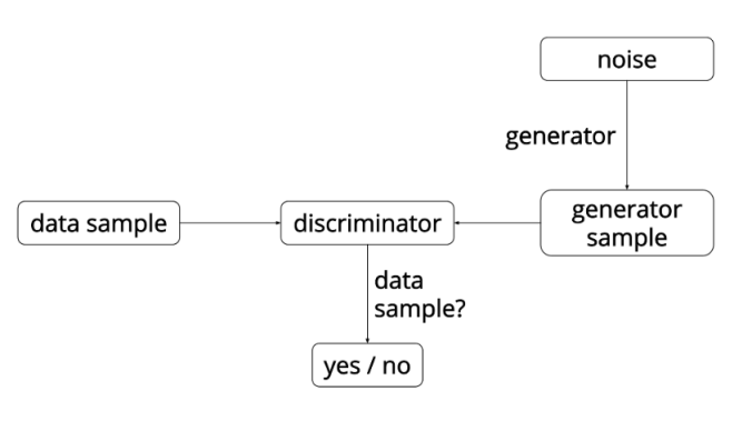
Figure – A basic architecture of Generative Adversarial Networks. Source  – http://blog.aylien.com/introduction-generative-adversarial-networks-code-tensorflow/

The discriminator is trained by providing it data form training set and the samples from generator and then back-propagating from a binary classification loss. The generator is trained by back-propagating the negation of the binary classification loss of the discriminator. The generator adjusts its parameter in such a way that the generated data cannot be discerned from real data by the discriminator. The ultimate goal is to find parameter settings such that discriminator is fooled.

GANs have been used in image domain to generate photorealistic images. They have also been used to generate the next frame in a video. More recently, GANs are used to reconstruct 3D models of objects from images. More recently GANs have also been used to generate sound and text.

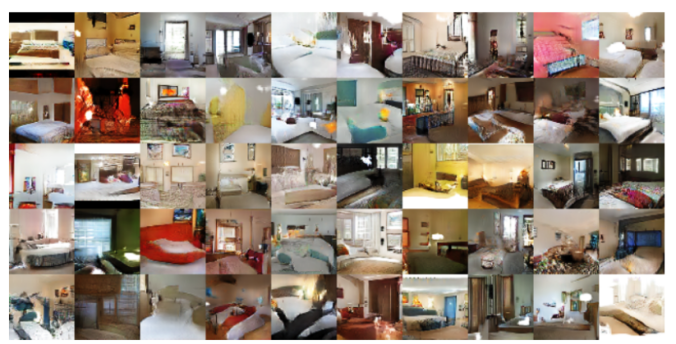
Figure – Bedrooms generated by GANs after training on bedroom images.

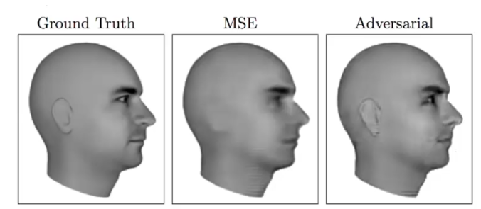
Figure – Comparison of MSE vs. Adversarial outputs. As clear, GANs produce a sharper image.

Few similar approaches to GANs

In my opinion, GANs are not an entirely new idea. The complete idea of GANs is based on a zero-sum game framework. Optimal strategy problems (A game between two players where both of them play optimally. Some problems can be found here.) have been known in the algorithms for a long time. Zero sum games have been explored in game theory and optimization problems. The novelty that GANs bring to the field is multi-dimensionality and incorporating neural networks.

This structure may also seem a bit similar to reinforcement learning where discriminator sends a reward signal to the generator letting it know the accuracy of the generated data. However, the key difference with GANs is that gradient information from discriminator is propagated to generator to improve it.

Auto-encoders also seem to be structurally similar to GANs. They have two neural networks. One of them the encoder produces a encoded representation and the other produces the decoded information from the encoded representation. The difference of auto-encoder from GANs is that here instead of competing both the networks work together to produce a model. Another difference is auto-encoders require labeled data.

A peak into the math

GANs are a kind of structured probabilistic models containing latent variables z and observed variables x.  The generator is a differentiable function G modeled as a deep neural network. Generator takes z as input and θ^(G) as parameters. Similarly, discriminator takes x as input and θ^(D) as parameters. The corresponding cost functions are  –

Discriminator – J^(D)(θ^(D),θ^(G)) and only θ^(D) is controlled.

Generator – J^(G)(θ^(D),θ^(G)) and only θ^(G) is controlled.

The main aim for all GANs is to minimize the discriminator cost function.

Discriminator cost function used in the original NIPS paper is defined as –

Toy Application

We borrow our strategy from the aylien post for 1-D gaussian distribution. We extend the methodologies to include multi-modal gaussians.

In this blog, we focus on three different modes – uni-modal, bi-modal and tri-modal gaussian distributions. The strategy is as follows –

1. We keep the discriminator function as is in the original blog.
2. The generator function used in aylien blog (without any changes) is very weak and takes about 4 hrs. to converge. We therefore make changes to the generator function so that the generator learns the training data distribution within 5000 steps.
3. Next, we see how the output dimensionality affects the number of steps taken.

Following are the main components of our GAN –

1. Data Distribution – A 1-D gaussian with 1, 2 modes. In this blog we use modes 1, 2 and 3.

Figure – Data Distribution showing Gaussian with 1 mode and 2 modes.

Next is the data distribution function. We try to keep the number of points in each Gaussian  to be equal. Thus, for multi-modal Gaussians, the number points from each distribution is almost equal.

This slideshow requires JavaScript.

Slideshow – The slideshow represents the three different data distributions used. To differentiate look at __init__. 1 (mu, sigma) pair means uni-modal, 2 means bi-modal and so on.

2. Discriminator – The discriminator in our example consists of three hidden layers, each of them performing a tanh activation after running a linear function on the input (input means input to this layer). Followed by this, we have a sigmoid output layer, to classify each data point as belonging to generator or real training data.

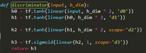
Figure – The discriminator function.

3. Generator – The most important component of our model is the generator. After spending many hours on tweaking the generator, I found an ideal combination of hidden layers that can generate good data for uni-modal, bi-modal and tri-modal Gaussian distributions within 5000 steps. The below slideshow presents the three different generators for three distributions.

This slideshow requires JavaScript.

Slideshow – The slideshow shows 3 generators. To differentiate see the second argument inside the linear function. h_dim is for uni-modal, h_dim*2 for bi-modal and h_dim*3 for tri-modal.

Note – We used the same gradient descent exponential optimizer as in the original blog and hence did not paste it here.

We have kept the size of the hidden layer for each of them as 4. Note the changes are the output dimensions for the linear function. The linear function multiplies the input with a generated w according to the formula wx+b (our old linear function). Below we present the output as generator and discriminator distributions for all cases.

Figure – The output of all three distributions. All three distributions converged much before our limit of 5000 steps. The uni-modal and bi-modal distributions converged within 20 – 30 steps and tri-modal within 300 steps.

The great peaks are not incorrect. It just means that the generator has identified the mean of the training data and is now generating most of the data around the mean.

You can click on the following links to watch the videos of the training steps. (The videos are very slow, so please fast-forward.)

1. Uni-modal
2. Bi-modal
3. Tri-modal

The interesting point is once we defined a common generator function, the time to converge remains constant if you increase the number of output dimensions “somewhat” linearly. The longer tails at Gaussian peaks for generator means the generator has learnt the distribution with a strong confidence and is producing data around its mean.

Support for our argument

I present some arguments of why I think our observations make sense. I present some facts observed over the course of the experiments performed.

1. If we remove one of the layers in generator for uni-modal distribution, the networks take more steps to converge. With the current generator (agreed that it is strong for uni-modal distribution) takes 20 steps to converge, however if one of the layers is removed it takes about 150 steps to converge, which is a 8 times increase.
2. For tri-modal distribution, with all linear functions with output dimensions multiplied by 3 we get the convergence at step 300. But if you reduce the output dimensions for two layers in generator as in below figure, we get a comparable convergence at step 3050 which is almost 2500 extra steps. For simplicity of math, assuming each step takes 1 second to run, it takes an extra 2500 seconds or 42 minutes. Just think of how an efficient generator can save time for generating more complex high dimensional models.

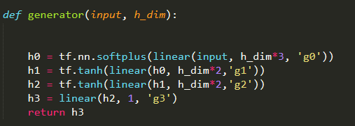
Figure – The generator with output dimensions reduced to h_dim*2 for last two hidden layers. This results in convergence pushed to 3050^th step instead of 300^th when all hidden layers have dimensions h_dim*3.

Conclusion

This blog presents two outcomes.

First, we present a stronger one-stop shop generator for multi-modal Gaussian distributions which converges within 5000 steps. There are two minute details to be considered here –

1. This generator is a one-stop shop generator given that the discriminator is not changed.
2. We mention 5000 steps keeping in mind that people would love to experiment on a distribution having 10 or 15 modes. Currently, with 3 modes, convergence is achieved at 300 steps. Saying that,

Second, we notice “almost” linear relationship between the output dimensions and number of modes in a distribution. Although we have done a basic experiment and it is too early to make commitments, but if through more experimentation, this trend proves to be correct, it can significantly improve the training time of GANs by giving data scientists an idea of what their generators must look like by first visualizing the training data.

Few Research Areas on GANs

1. Issue of Non-Convergence – One of the biggest research areas related to GANs is the issue of non-convergence. Although I do not possess sufficient skills to delve on that, I visualized a first hand case of this. If you recreate the Gaussian 1-D experiment from here, the generated data does not converge with the real data. Since it uses gradient descent, finding a suitable learning rate is important. However, what I noticed is once the random_seed is changed to 4 instead of 42, the models converge which is strange.
2. Evaluation – There is no way of quantitatively evaluatinig a GANs or generative models in general. Models that have good likelihood may generate bad samples or vice-versa. GANs evaluation is much more difficult because of the difficulty in estimating their likelihood.

References

1. NIPS 2016 Tutorial: Generative Adversarial Networks, Ian Goodfellow – https://arxiv.org/pdf/1701.00160.pdf
2. Introduction to Generative Adversarial Networks – http://blog.aylien.com/introduction-generative-adversarial-networks-code-tensorflow/
3. Generative Models – https://en.wikipedia.org/wiki/Generative_adversarial_networks
4. Discriminative Models – https://en.wikipedia.org/wiki/Discriminative_model